systems physiology · computational modeling

Simulating the circulation, then closing the loop on it

A lumped-parameter model of the human cardiovascular system in MATLAB, used first to trace an injected solute through thirteen compartments, then extended into a closed-loop respiratory controller and pushed off balance to see whether it recovers. Built with Easa.

Solute transport

The base model divides the body into thirteen compartments — lungs, brain, heart, liver and GI, kidneys, muscle, skin, bone, fat, thyroid, sex glands, adrenals, and a catch-all — each with its own volume, resistance, compliance, and inertance, plus arteries and veins. A four-chamber heart with time-varying elastance and pressure-driven valves supplies the flow.

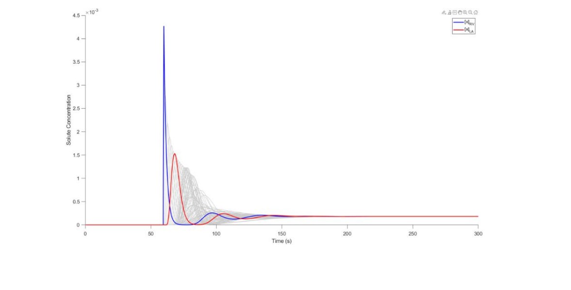
The first question the model answers is whether pulsatility matters. One unit of solute is injected and tracked as it circulates, run twice: once with the heart actually beating, and once replaced by steady flow.
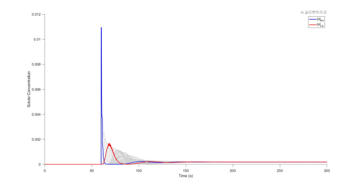
Solute concentration over time across all compartments for the beating heart condition
Beating heart. First pass through the right ventricle, then the lung transit peak, then recirculation.
Solute concentration over time across all compartments for the constant flow condition
Constant flow. Same overall shape, roughly a quarter of the peak concentration.
MeasureBeating heartConstant flow
Compute time18.9 s1 s
Final solute concentration0.00018790.00018134
Lung mean transit time8.52 s8.5 s
First recirculation peak, right ventricle41.62 s37 s

The useful result is the trade. Pulsatility costs roughly nineteen times the compute and buys almost nothing on the slow measures: mean transit time through the lungs differs by two hundredths of a second, and both conditions converge on the same well-mixed final concentration, which checks out against one unit distributed across total blood volume. Where it does matter is recirculation timing, which arrives about five seconds later with a beating heart, and peak amplitude, which is far higher. So if the question is steady-state distribution, constant flow is the right model; if it is peak exposure or arrival timing, it is not.

Watching the animation, the fast compartments are the ones you would expect from perfusion per unit mass — heart, brain, kidneys, thyroid, adrenals. Bone, fat, and the catch-all are slowest in both conditions.
The control loop

Part two turns the open transport model into a closed-loop physiological controller. Carbon dioxide is generated by every tissue in proportion to its blood supply, carried by the same transport machinery, and cleared only at the lungs. The clearance rate is not fixed — it is set by the controller, which makes the whole thing a negative feedback loop.

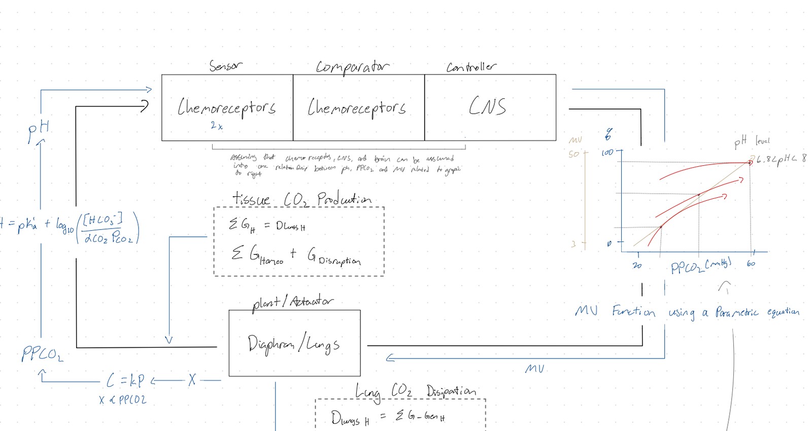
Mapped onto control-system blocks: the chemoreceptors are the sensor and comparator, the CNS is the controller, and the diaphragm and lungs are the plant. Partial pressure of CO2 goes in, pH comes out of the Henderson-Hasselbalch equation, and minute ventilation comes out of a parametric function fitted to the physiological pH–PPCO2–MV relationship. Ventilation then drives depletion at the lungs, D = PPCO2 × 0.005 MV, which feeds back into the CO2 the tissues are still producing.

Hand-drawn control system block diagram of the CO2 and pH feedback loop
The loop drawn as control blocks, with the governing equations and the fitted minute-ventilation surface.

The ventilation function itself is a three-point parametric fit through the clinical relationship, anchored at 30 mmHg / pH 7.52 / 11 L·min⁻¹ and 50 mmHg / pH 7.15 / 43 L·min⁻¹. Homeostatic targets are a PPCO2 of 25 to 45 mmHg, a pH of 7.4, and minute ventilation between 3 and 50 L·min⁻¹.

Disturbance response

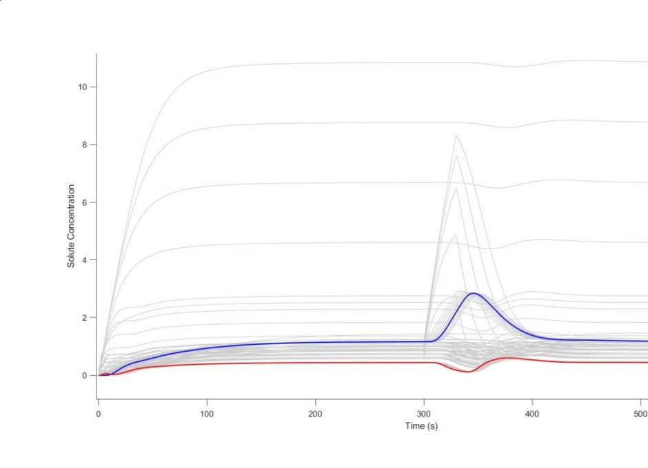
A model of a controller is only worth as much as its response to being knocked off target, so the loop is disturbed at t = 300 s with a simulated vomiting episode: acid is lost from the liver and GI compartment, producing metabolic alkalosis and a step rise in CO2 in that tissue.

Simulation output showing the disturbance at 300 seconds and the return to homeostasis
Disturbance at t = 300 s. Grey is the actual signal, blue the measured signal at the right ventricle, red the command signal.

Transport delay from the disturbance to the measured signal is 10 seconds, and to the command signal another 10 — the time it physically takes disturbed blood to reach the chemoreceptors and for the response to reach the lungs. The loop then settles back to its pre-disturbance values over a homeostatic time constant of roughly 100 seconds, with no sustained offset and no oscillation. The controller is stable and the delays are the ones circulation time would predict.

The code

Around 1,900 lines of MATLAB across six files. Compartment properties load from a CSV rather than being hard-coded, so the body can be re-partitioned without touching the solver.

FileRole
HW_03_SystemsPhysiology.mMain simulation: heart activation functions, valve mechanics, hemodynamics, time stepping
HW_03_construct_branches.mBuilds the circulatory network from the compartment list
HW_03_construct_coefficient_matrixes.mAssembles the system matrices for each time step
HW_03_solute_transport.mFlux across every connection, sign-aware for flow direction, forward Euler step
HW_03_MV_Function.mMaps PPCO2 and pH to minute ventilation
pH_PPCO2_MV_graph_and_linerized_function.mFits and plots the three-point ventilation relationship

The transport routine is the core of it. For each connection it reads the flow, checks the sign to decide which compartment is upstream, computes the flux as concentration times flow over volume, and applies it as a loss to one compartment and a gain to the other. Handling the sign explicitly is what lets the same routine serve both the systemic tissues and the reversed pulmonary path.

Keywords

computational modeling MATLAB systems physiology control systems hemodynamics numerical methods

Full report

Transport results, the system description, the control block diagram, and the disturbance analysis.

Download PDF

MATLAB source

All six scripts plus the compartment parameter table.

Download ZIP